Uniswap Multipool
Intro
In this paper we are looking at the dynamics of what happens in the presence of multiple Uniswap-style pools that are trading the same tokens. In our example the tokens we trade are called X and Y. We generally consider X to be the active token, ie whoever interacts with the pool chooses what happens with X and then the pool reacts accordingly with the token Y. This of course does not correspond to the technical reality where one has to send one of the tokens into the pool contract, and the contract returns the other token in the appropriate amount.
We are not providing any of the formulas here. Instead we refer the reader to our Uniswap formula paper. Please also note our convention that all signs are considered from the perspective of the pool, so a negative change in token X, $dx<0$, means that the pool pays out tokens of type X and receives those of type Y and vice versa.
The single and multi-pool charts
Introducing single pool charts
The charts are pretty dense in terms of information content, so we want to introduce them slowly. We therefore start with a single pool, and we only add the second pool once the meaning of the single pool charts is clear.
The multi-pool charts are somewhat easier to understand when the two tokens are currently valued the same. However, it is worth understanding how the charts look at a generic exchange ratio first, so before moving on to an exchange ratio at par we start with an exchange ratio of 1 X being worth 4 Y.
Single pool at price of 4
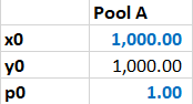
The table below shows the initial parameters of the pool: it contains 1,000 tokens of type X and 4,000 tokens of type Y. The pool is currently arbitraged, so we assume that this is also the fair exchange ratio X vs Y, even though we initially do not need this assumption.

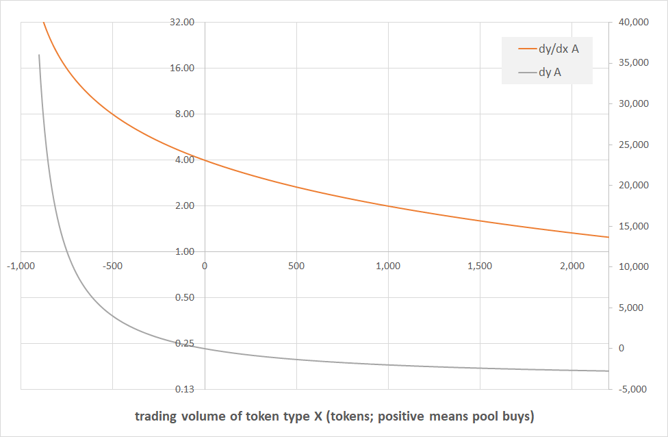
Our first chart shows that transaction volume (grey; RHS axis) and effective exchange ratio (orange; LHS axis) as a function of the number of tokens of type X ($dx$) contributed to the pool ($dx>0$) or withdrawn from the pool ($dx<0$).
Let’s look at the grey curve first, ie the transaction volume, as a function of the number of tokens contributed to / withdrawn from the pool $dx$. The first thing to note is that for $dx=0$ the amount of tokens withdrawn $dy$ is also $0$, which is unfortunately somewhat hard to see as the relevant value is on the secondary axis and there is no guiding line. Let’s first consider what happens when we want to buy tokens of type X from the pool, ie $dx<0$. We see that if we go towards the left the curve becomes very steep, meaning we have to pay a lot of tokens of type Y into the pool if we want to go there. This makes sense, as the pool has only 1,000 tokens of type X, and it “protects itself from being depleted” by having the price of those tokens explode when we get close to the 1,000 mark.
We then look at what happens when we contribute tokens of type X to the pool, ie $dx>0$. In this case the curve gets flatter and flatter as the more tokens of type X we contribute the pool, the fewer tokens of type Y we get back. Of course if we were to look at this from the point of view of token Y we would see exactly the same peek that we described at the paragraph before, and the fact the $dx<0$ looks different from $dx>0$ is simply due to us looking at the world through the lens of token X.
The second, orange, curve on this chart is the effective price curve, ie it measures how many tokens of type Y, $dy$, we got for our tokens of type X, $dx$. Note that despite our notation the term $dy/dx$ is not a derivative, it is simple the ratio of two numbers. The first thing we see here is that for $dx\approx 0$ the exchange ratio is 4, ie the ratio of tokens in the pool. If we want to remove assets of type X from the pool then we need to pay more than 4 Y-per-X, and if we contribute X to the pool then we get fewer than 4 Y-per-X. Again, we see that the the pool “protects itself” and for $dx \to -1,000$, ie the total number of tokens of type X in the pool, the price becomes infinite, so we’ll never able to remove them all. Similarly, for $dx \to +\infty$ the price we receive goes towards zero, so again, regardless how many tokens of type X we put into the pool we are never able to remove all tokens of type Y.
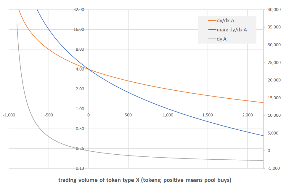
The next chart finally shows the same data as before, plus we added the marginal price. As a reminder, $dy/dx$ is the ratio of total Y received/paid in exchange for the X, divided by the total amount of X. This term is not a derivative. In this chart however we added the derivative of the price function in blue, referred to as marginal $dy/dx$. In other words, that is the marginal amount of Y that we receive for the “last” token of type Y we contributed to the pool, pr vice versa. We set that for $dx \approx 0$ the marginal price equals the average price equals the pool exchange ratio, and then in both directions it moves more strongly than the average price. No surprises here – that is what marginal prices do.
Single pool at price of 1
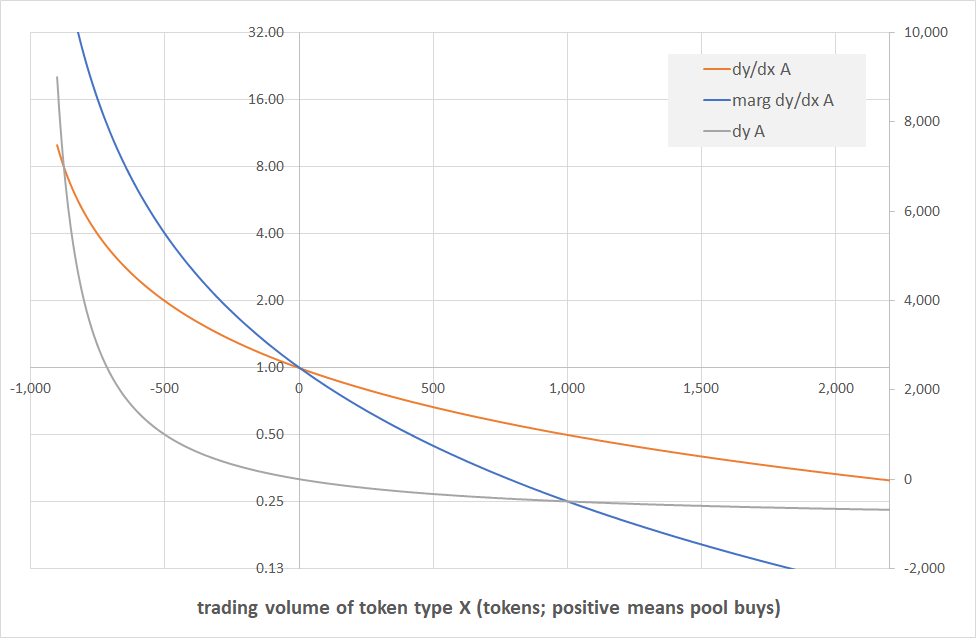
Having looked at a single pool at an exchange ratio of 4 we now look at an exchange ratio of 1, ie initially our pool contains 1,000 tokens of each kind.
The charts look exactly the same as above, the only difference being that now both the marginal and the average price for $dx \approx 0$ are 1 instead of 4.
Introducing multi-pool charts
Havinf discussed single pool charts we now move to multiple-pool charts, or more precisely two-pool charts. Our exchange ratio is at 1, and the pool A is exactly as above, with 1,000 tokens of each. Pool B is 50% bigger, and is contains 1,500 tokens of each type.
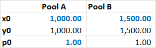
Full chart
Let’s dive into the full chart first. This corresponds exactly to the three-line single-pool chart above, ie the grey lines are the amounts exchanged, the orange lines are the average prices, and the blue lines are the marginal prices. In fact, the solid lines are exactly the lines from the chart above. The only difference here are the dashed lines which corresponds to the equivalent quantities in the second, bigger, pool.
We won’t see the grey line again, so let’s look at this one first. We see that the dashed line is somewhat flatter than the solid one, and it seems to react more violently in both directions. This makes sense of course: the Pool B contains 1,500 tokens of each type, compared to the 1,000 in Pool A, so when Pool A starts panicking towards $dx \to -1,000$, Pool B can still remain somewhat calm. The same happens in the other direction.
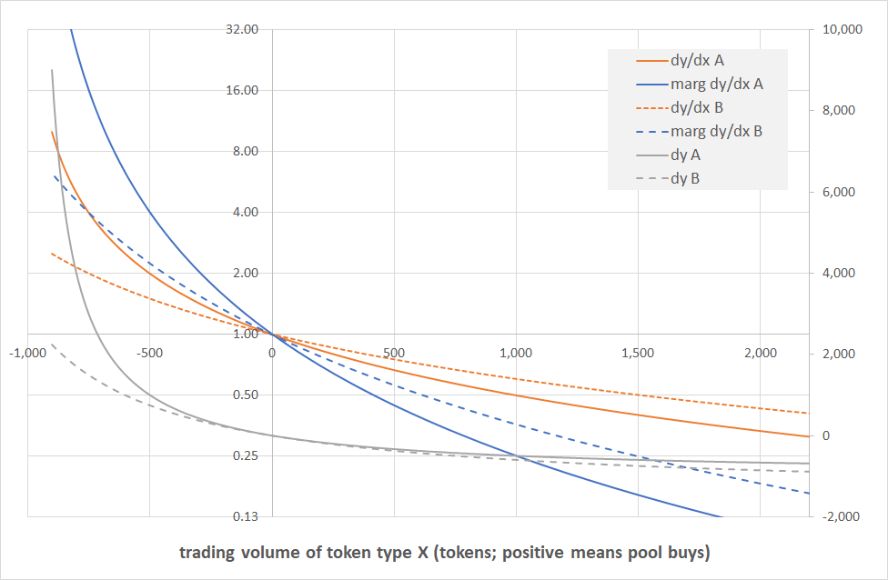
Price charts
Now the grey curves are nice, but not particularly useful, so we removed it here and look at the price charts only. Other than that the chart is just like the chart above, ie the two orange and the two blue lines are exactly the same.
We here see what we have already seen on the grey lines which is that Pool B reacts less violently than Pool A, and therefore its (dashed) price curves are flatter than those (solid) of Pool A, both for average (orange) and marginal (blue) prices. We also see that all curves meet for $dx \approx 0$ at the pool exchange ratio which here is 1.
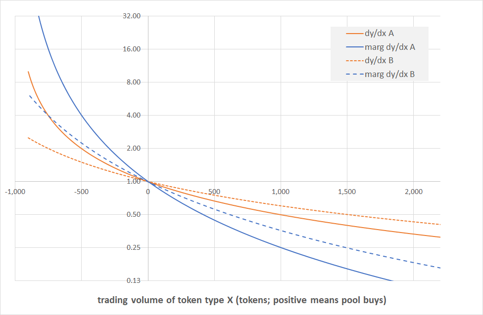
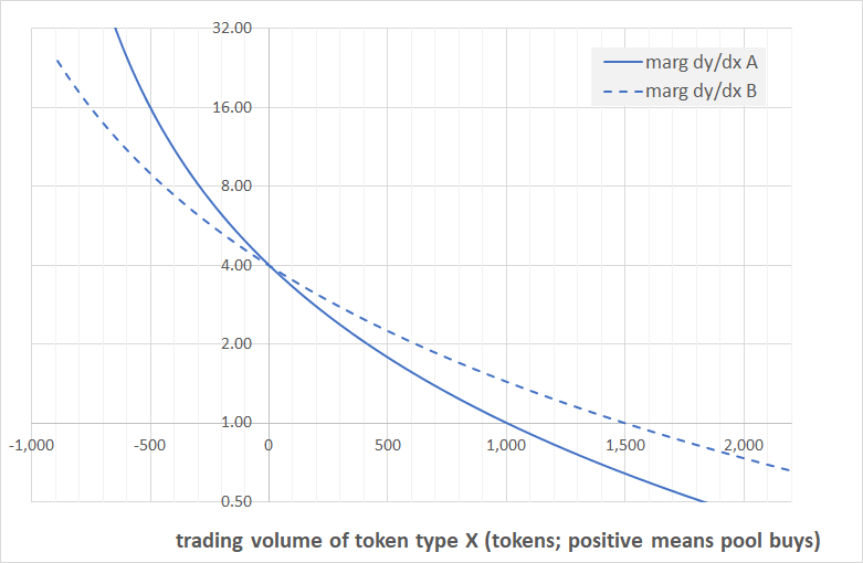
Last but not least we are showing the chart of the marginal prices only. Again, this is not new information, those blue lines are exactly the same lines as in the two charts above. The only reason why we are showing them on their own is because in what follows the marginal prices will be the only prices we consider, and so we want to make sure we have the correct context here.
Multi-pool analysis
After having done the groundwork explaining the charts we can now move on to acutally using them to analyse what happens in world where there are multiple pools with the same constituents on the same chain. This might not be possible in say a Uniswap-only setting as the system might not allow to create a second liquidity pool with the same constituents as one that already exists. However, as we have seen in the Sushiswap story, it is always possible to fork the protocol and to create multiple equivalent pools within nominally different protocols.
The most important insight in this paper – and ultimately the reason why we went through the entire analysis and explanations above, is the following:
Propostion 1 (optimal pool routing). In the absence of fixed transaction costs, and in the presence of multiple pools that trade the same token pair, rational market participants will route their orders to all available pools in a manner that the marginal trading prices in all pools is the same.
Proof. Firstly, because of the absence of fixed transaction costs, routing an order to multiple pools is costless. The costlessness even holds in presence of proportional transaction costs as in this case routing does not change the overall fee, it merely change its apportionement. The equalisation-of-marginal-prices arguments is a well-rehearsed argument in micro-economics. Essentially if the marginal pricing was different between the routable pools then marginal volume would be withdrawn from the more expensive pools and reallocated to the cheaper ones. The only situation where this reallocation of volume can not happen is where all marginal prices are equalised. QED.
To see what this means we look again at our marginal price chart. We are back to an exchange ratio of 4 (we do not want to introduce spurious egalities because of an exchange ratio of 1), and the pool sizes for token X are 1,000 and 1,500 respectively.
We found above that to understand pool routing we have to look at equalising the marginal trading prices between the different pools. In our chart this corresponds to horizonal lines, and each of the thin red lines on the chart corresponds to one specific price level.
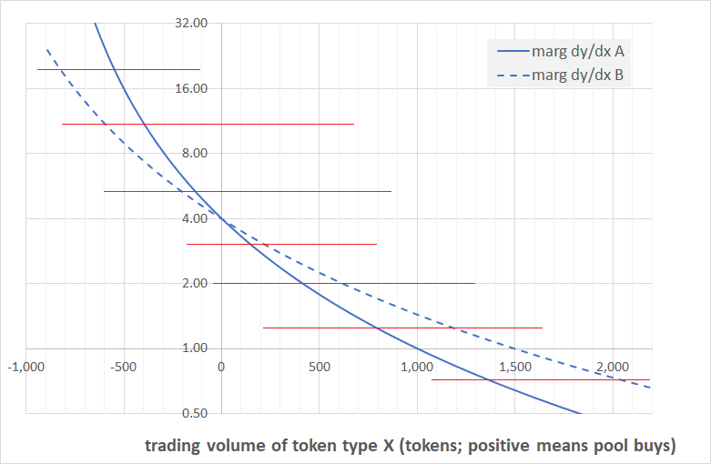
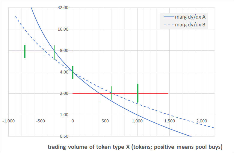
To find the corresponding volume to a given price level we need to add up the volumina of the constituent pools. We have shown this for the price levels of 2, 4, and 8 in the chart below. The pools are all arbitraged at a price of 4, so at exactly this price the trading volume available is zero. At a price of 2 X-per-Y, the two pools are willing to buy 400 and 600 tokens of type X respectively, leading to a total volume of 1,000. At the price of 8, the pools are willing to sell 300 and 450 tokens respectively, leading to a total available volume of 750.
We next come to the central proposition of this paper. Technically it is still a conjecture of course, but we are highly confident it is correct.
Conjecture 2 (pool aggregation). If we have multiple pools with all parameters identical except for the size then under optimal routing as described above those pools behave identical to a large pool of the aggregate size of the underlying pools.
Proof. As the formulas are known we are confident that this conjecture can be proven, but we did not get around to it yet. Also it our hunch that there is a very elegant proof based on scale invariance that we could not yet formulate, and rather than going through the tedious task of working through the details of the formulas we are waiting for inspiration on the scale proof. There are however a number of pointer that this conjecture is correct. Firstly it works at both boundaries: the pole of the aggregate pool where prices go to infinity is at the sum of the poles of the underlying pool (the location of the poles corresponds to the number of the tokens in a pool). It also holds in the center as can easily be seen when doing a linear approximation of the curve.
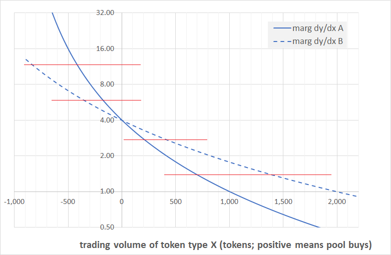
Last but not least, the conjecture seems to hold numerically, as shown in the chart below. By way of explanation, in this case Pool B (dotted line) is 2,000 tokens whilst Pool A (solid line) is 1,000 tokens. As we can easily see at the grid lines as well as the red lines drawn on the chart, at the same price the trading capacity of the bigger pool is excactly twice that of the smaller one. In other words: the trading capacity of the pool twice as big is the same as that of two pools. QEFD.
This finally leads us to the most important economic result of this paper, which is the following
Corrolary 3 (lack of scale economies). With no fixed transaction costs there are no economies of scale within a Uniswap framework, in the sense that whilst it is true that a bigger pool trades more efficiently than a smaller one, multiple pools of the same aggregate size as a bigger one trade, under optimal routing, as efficient as that bigger one.
Proof. This is simply a restatement of Conjecture 2 above. QED.
Conclusion
To some extent we decided to stop this paper just when it became interesting, but other than providing a nice cliff-hanger there is some logic to it: in this paper we went as far as we needed to on the mathematical side of things [editor’s note: you could have proved the conjecture]. What follows now is economics, and by and large all we need for the economics paper is the Corrolary 3. So instead of scaring off everyone with scary looking charts we will continue this discussion in a new paper that takes Corrolary 3 as given, and takes on the economics discussion from there.
Be that how it may, let’s discuss what we have shown in this paper. We built on the formulas contained in the formula paper to draw some graphs what exchange ratio a Uniswap pool provides, in function of the trade size and the number of tokens in the pool. We showed that for very small trades the exchange ratio is equal to the ratio of tokens in the pool, and that it worsens on either side of that. In fact it worsens so much – the price going to infinity at the pool capacity – that it is never possibly to empty the pool of one of the tokens by trading.
The most important finding of this paper [editor’s note: conjecture; you meant to say conjecture!] is that a collection of small pools that are identical except for their size behave like a big pool whose size is the aggregate size of the constituent pools. This results holds under a number of very weak conditions, notably the absence of fixed transaction costs (or at least, that those costs are de minimis compared to the pool size) and that user use “optimal routing” (as described in Proposition 1) to place their rates.
This conclusion is very important, and will be the subject of a forthcoming more economics-focused paper. In a nutshell this means that there are no economies of scale for large pools. We will show in the forthcoming paper that this has massive implications for the profitability of the pool operations, and therefore for the value that can be captured by liquidity providers and protocol token holders.